Orbital Dynamics & Numerical Analysis: Satellite Path Modeling

TL;DR

Developed a robust, modular MATLAB suite designed to determine critical orbital parameters—specifically size ($C$), eccentricity ($e$), and phase angle ($\alpha$)—based on three sets of observations $(R, \theta)$. The architecture leverages the Newton-Raphson method to linearize non-linear equations and provides multiple computational pathways for solving the resulting systems, including Cramer’s Rule, Gauss Elimination with Partial Pivoting, and Naïve Gauss-Jordan.

Problem

The motion of a satellite orbiting Earth is typically modeled as an ellipse in polar coordinates. The governing equation for this orbital path is defined as:

$R = \frac{C}{1 + e \sin(\theta + \alpha)}$

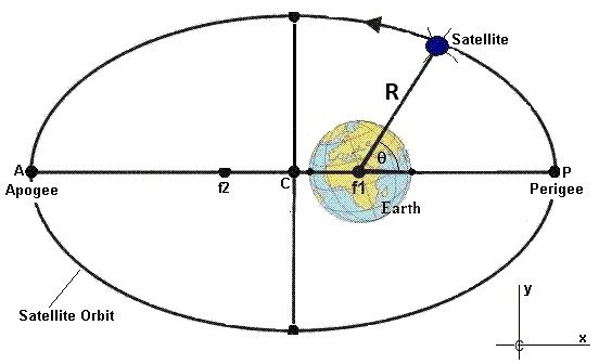
While this equation defines the orbital path, the constants $C$, $e$, and $\alpha$ are initially unknown. To determine these values, the system must solve a set of three non-linear equations derived from three distinct observation points.

The primary engineering challenge was to transform these non-linear equations into a solvable linear system while maintaining numerical stability and providing the user with multiple algorithmic pathways to verify calculation accuracy.

Design Iterations

To ensure high-fidelity results, the system was engineered using a multi-layered approach:

1. Linearization: The Newton-Raphson method was implemented to iteratively linearize non-linear equations, allowing the system to converge on the correct orbital constants through successive approximations.
2. Solver Versatility: To ensure robustness and provide cross-verification, the software offers three distinct methods for solving the resulting linear systems:
   • Cramer’s Rule: Utilized for direct determinant-based calculation.
   • Gauss Elimination with Partial Pivoting: Implemented to mitigate rounding errors by swapping rows to ensure the largest pivot element is utilized during elimination.
   • Naïve Gauss-Jordan: Employed to transform the coefficient matrix into an identity matrix for direct solution extraction.
3. Validation Logic: A Bisection Method was integrated as a secondary tool to predict the angle $\theta$ for a given radius $R$, providing an independent check on the precision of the calculated orbital constants.

Technical Details

The software architecture is strictly modular; each numerical method is encapsulated within its own function to ensure maintainability and clarity.

• Newton-Raphson Implementation: The core engine calculates partial derivatives for $C$, $e$, and $\alpha$ to construct the Jacobian matrix, which is then used to update estimates in each iteration.
• Error Tracking: A dedicated calculation module, Approx_Relative_Error, monitors the percentage change between iterations, ensuring the system only terminates once the user-defined convergence criteria are met.
• Robustness via Pivoting: Within the Gauss Elimination module, partial pivoting was implemented to handle potential zero-division errors and minimize precision loss during the elimination phase.

Results & Key Metrics

The system successfully produced high-fidelity orbital data, validated through two primary visualization methods:

1. Error Analysis Plots: The software generates a plot of the relative error for $C$, $e$, and $\alpha$ against the number of iterations, demonstrating rapid convergence toward target values.
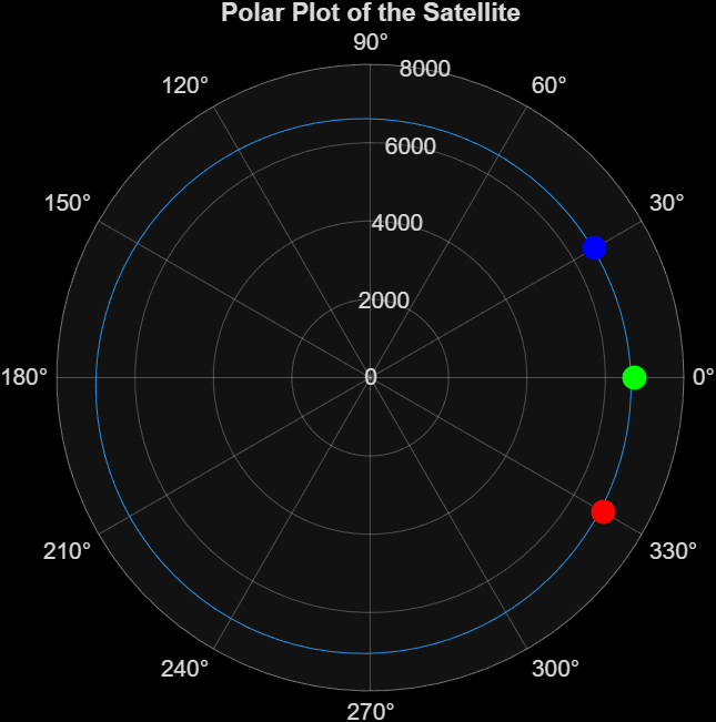
2. Polar Plot Visualization: A final polar plot maps the orbit, overlaying the three original observation points to visually confirm that the calculated parameters accurately represent the physical path of the satellite.

Frameworks & Tooling

MATLAB Computation