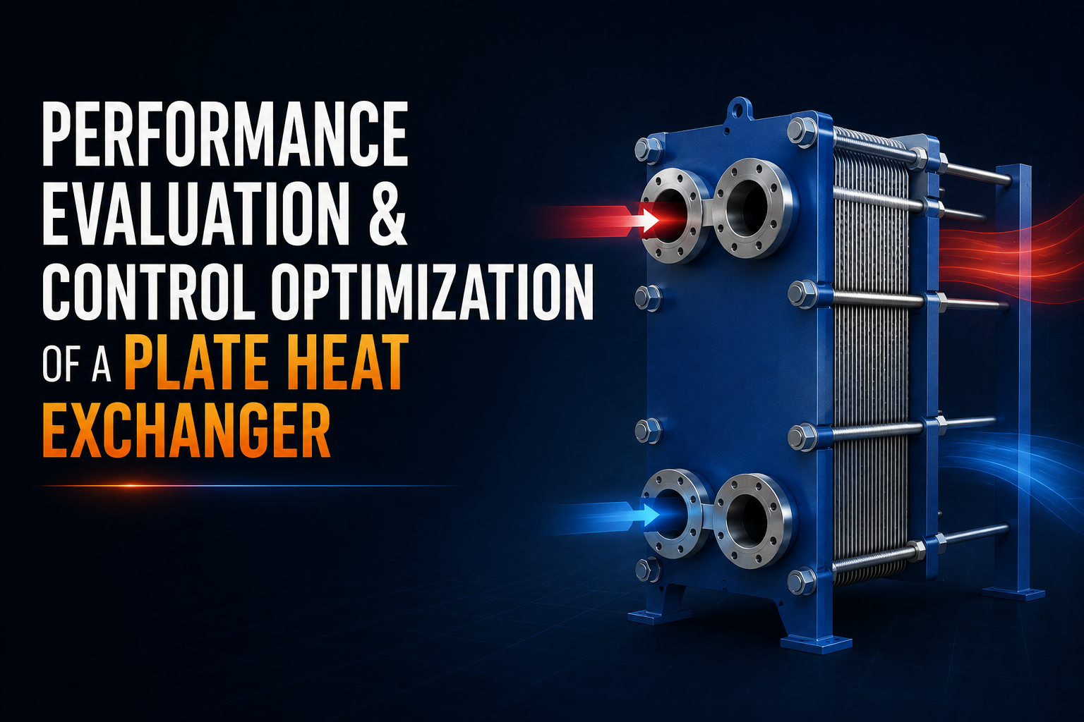
TL;DR

This project focuses on the high-fidelity dynamic modeling, thermal evaluation, and feedback control optimization of a counterflow gasketed Plate Heat Exchanger (PHE)—a core thermal management unit used in district heating, chemical processing, and power generation.

By comparing a two-degree-of-freedom $H_{\infty}$ loop-shaping control strategy against a discretized Cell Division Lumped Parameter Model, I led the derivation of first-principles state-space transfer functions that dynamically integrate thermal fluid dynamics (Reynolds, Prandtl, and Nusselt numbers) alongside motorized valve actuator dynamics. Implementing an optimized PID feedback controller in MATLAB and Simulink reduced system settling time by 6.3% and rise time by 5.3%, maintaining zero overshoot while adhering strictly to physical actuator saturation limits and thermal gradient safety constraints.

Background & System Architecture

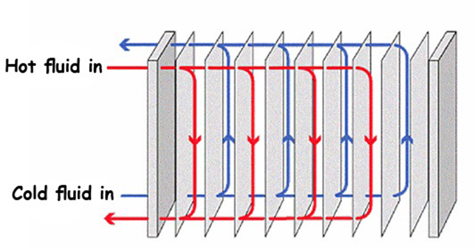
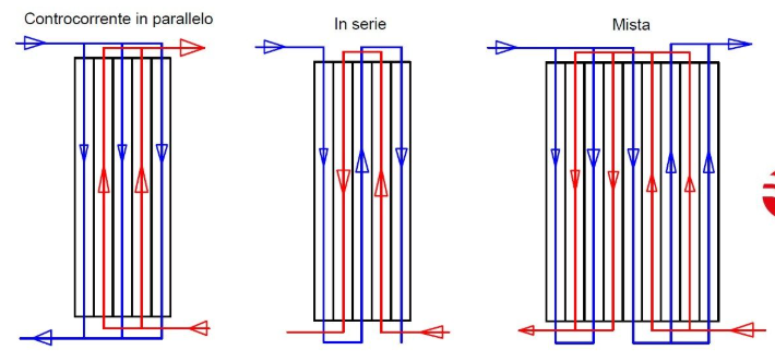
Plate heat exchangers transfer thermal energy between two fluid streams across a sequence of corrugated metal plates clamped between fixed and pressure frames. In industrial district heating and HVAC systems, precise secondary-side outlet temperature regulation is paramount for energy efficiency and structural longevity.

❮

🔍 Click to expand

🔍 Click to expand

🔍 Click to expand

❯

✕

Physical System Parameters

The system evaluated in this study models a full-scale industrial counterflow PHE operating under district heating conditions:

Problem & Engineering Challenges

Regulating fluid outlet temperatures in a PHE poses non-trivial control engineering challenges:

1. Distributed Boundary Parameters: The governing thermal distribution is continuous in space and time, described by partial differential equations (PDEs) with high coupling between fluid streams.
2. State-Dependent Heat Transfer Coefficients: The overall heat transfer coefficient ($U$) is not constant; it dynamically varies with fluid velocity, thermal conductivity, and dynamic viscosity across operating temperatures.
3. Actuator Non-Linearities: The primary flow control mechanism—a motorized control valve—exhibits linear behavior only up to a $50\%\text{--}60\%$ opening angle ($60\text{ kg/s}$). Operating past this threshold introduces heavy saturation and gain degradation.

Operational Constraints & Assumptions

• Constraints: Mass flow rates restricted to $0.06\text{ m}^3\text{/s}$ ($60\text{ kg/s}$) to retain quasi-linear valve response; step-response settling time capped at target threshold to avoid thermal stress shocks; control effort tuned to prevent cavitation or hydraulic instability.
• Assumptions: Fluids are incompressible; ambient heat losses are negligible; phase changes do not occur; axial heat conduction within fluid streams is negligible relative to convective transport.

Comparative Modeling Methodologies

To establish an accurate control plant, two mathematical modeling frameworks were investigated and derived.

Approach 1: Finite Volume PDE State-Space Modeling ($H_{\infty}$)

The fundamental energy balance governing continuous temperature profiles along flow length $x$ for hot ($T_h$) and cold ($T_l$) fluid channels is given by:

$\frac{\partial T_h}{\partial t} = -\frac{q_h}{M b d} \frac{\partial T_h}{\partial x} + \frac{k}{\rho c_p d} (T_l - T_h)$

$\frac{\partial T_l}{\partial t} = \frac{q_l}{M b d} \frac{\partial T_l}{\partial x} + \frac{k}{\rho c_p d} (T_h - T_l)$

Using the Finite Volume Method (FVM) with upwind spatial discretization over $N$ control volumes:

$\frac{d T_{h,j}}{d t} = \frac{N q_h}{M b d L} (T_{h,j+1} - T_{h,j}) + \frac{k}{\rho c_p d} (T_{l,j} - T_{h,j})$

$\frac{d T_{l,j}}{d t} = \frac{N q_l}{M b d L} (T_{l,j-1} - T_{l,j}) + \frac{k}{\rho c_p d} (T_{h,j} - T_{l,j})$

This formulation constructs a high-order state-space model ($\dot{\mathbf{x}} = \mathbf{A}\mathbf{x} + \mathbf{B}\mathbf{u}$), enabling two-degree-of-freedom $H_{\infty}$ loop-shaping controllers ($K_1(s), K_2(s)$) to manage worst-case parametric uncertainties:

$K_1(s) = \frac{125.7 s^2 + 67.38 s + 6.586}{s^3 + 4638 s^2 + 331.4 s + 9.703}$

$K_2(s) = -\frac{7822 s^2 + 8724 s + 656.5}{s^3 + 4639 s^2 + 6022 s + 778.3}$

Approach 2: Cell Division Lumped Parameter Model (Selected Approach)

While $H_{\infty}$ handles structural uncertainties, the Cell Division Modeling Method was selected for full system simulation and controller optimization due to its direct mapping of physical fluid parameters into explicit transfer functions.

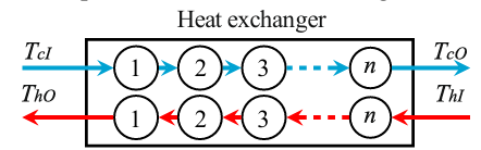
Each cell $j$ undergoes localized dynamic heat accumulation ($Q_s = \rho V c_p \dot{T} = Q_i - Q_t$):

$m_h c_{ph} \dot{T}_{h2} = \dot{m}_h c_{ph}(T_{h1} - T_{h2}) - U A (T_{h2} - T_{c2})$

$m_c c_{pc} \dot{T}_{c2} = \dot{m}_c c_{pc}(T_{c1} - T_{c2}) - U A (T_{c2} - T_{h2})$

Motorized Valve Dynamics & Actuator Integration

Controlling a physical heat exchanger relies on modulating a motorized valve position ($O_v$). The valve dynamics are modeled as a first-order lag relating valve opening percentage to hot fluid mass flow rate:

$\frac{\dot{m}(s)}{O_v(s)} = \frac{90}{0.1 s + 1}$

Combining actuator lag with plant dynamics yields the overall single-input single-output (SISO) control transfer function $G_1(s) = \frac{X_2(s)}{O_v(s)}$:

$G_1(s) = \frac{2213000}{s^3 + 205.3 s^2 + 9155 s + 72010}$

Simulation & Open-Loop Response Verification

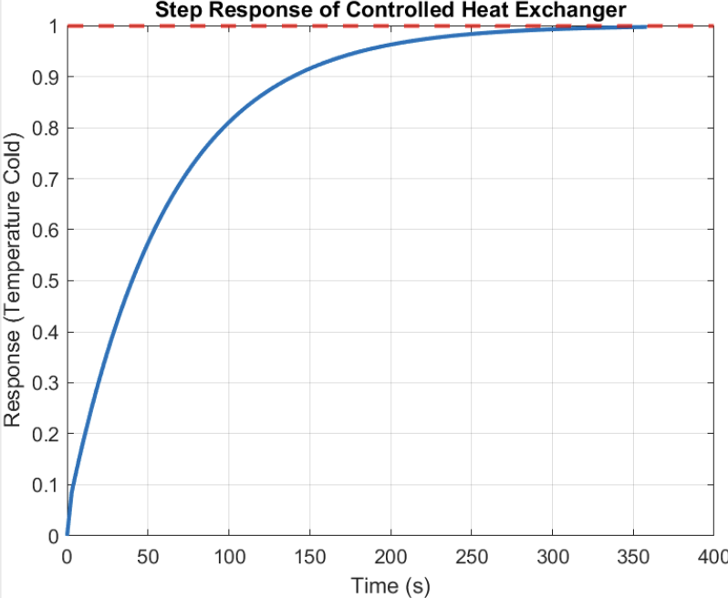
The derived plant transfer function $G_1(s)$ was evaluated in MATLAB under a step input corresponding to nominal hot stream flow manipulation.

MATLAB Step-Response Analysis

The open-loop system exhibits overdamped characteristics with high fidelity, matching verified physical benchmarks in published literature within a $1.083\%$ error margin.

Control System Design & Optimization

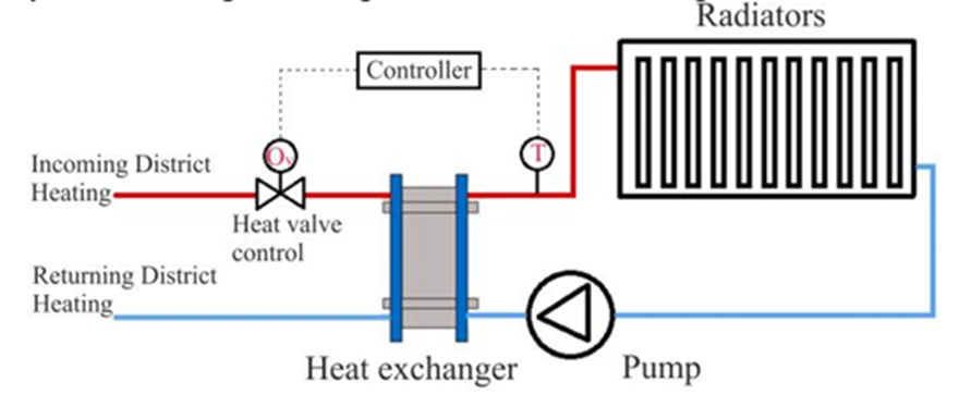
To maintain precise cold outlet temperature setpoints ($45.0^{\circ}\text{C}$) in the presence of load disturbances, a closed-loop feedback control system was modeled in Simulink.

❮

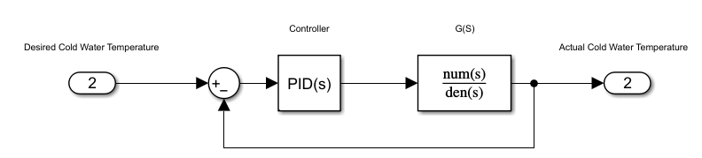🔍 Click to expand

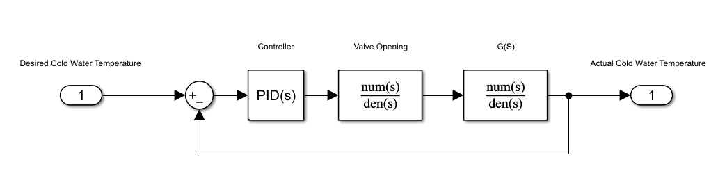🔍 Click to expand

❯

✕

Baseline vs. Enhanced PID Parameter Tuning

Literature baselines utilized conservative Proportional-Integral (PI) control ($K_p = 0.00015, K_i = 0.0005$) to avoid thermal strain. Through iterative pole placement and control loop shaping in Simulink, I developed an enhanced PID configuration ($K_p = 0.0015, K_i = 0.00055, K_d = 0.00014$).

❮

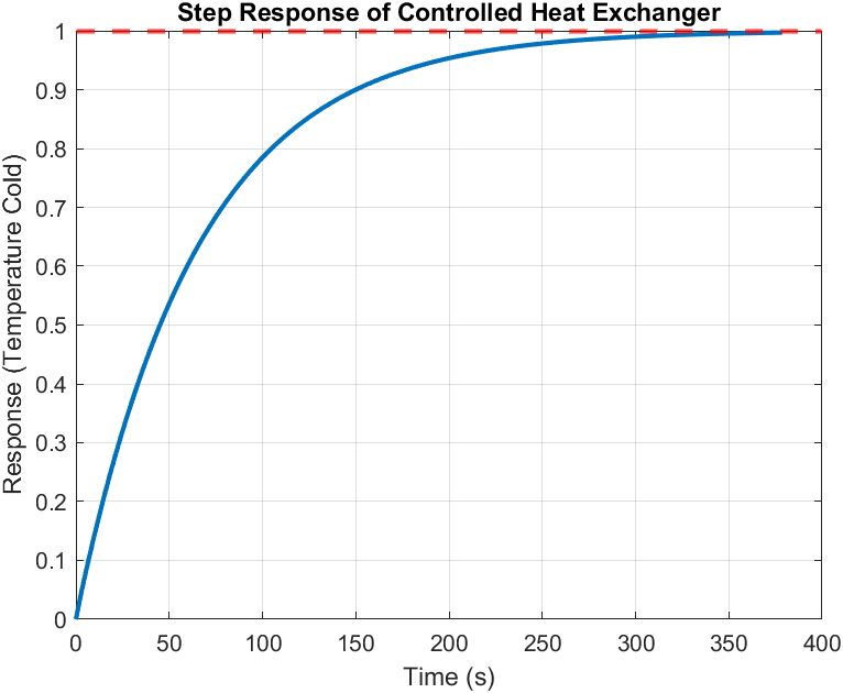🔍 Click to expand

🔍 Click to expand

❯

✕

Performance Optimization Summary

Practical Engineering Considerations & Ethics

1. Actuator Protection & System Integrity: Rapid control loops can demand aggressive flow transitions, inducing water hammer phenomena or excessive pressure drops across corrugated plates. The optimized PID gains enforce a smooth valve actuation profile, respecting the physical rate limits of motorized actuators.
2. Energy Efficiency & Decarbonization: Plate heat exchangers are central to district heating networks. Optimizing settling speed and thermal stability directly minimizes fuel consumption in primary boiler systems, reducing greenhouse gas emissions.
3. Reproducibility & Rigor: First-principles modeling ensures all thermal fluid properties ($\rho, \mu, c_p, k$) are mapped transparently across operating temperature steps ($40^{\circ}\text{C}\text{--}45^{\circ}\text{C}$), preventing over-fitting.

Limitations & Future Work

• Operating Point Sensitivity: Fixed-gain linear controllers exhibit performance degradation when moving far from nominal setpoints ($45^{\circ}\text{C}$) due to continuous shifts in fluid viscosity and $U$.
• Future Work:
  1. Gain Scheduling / Adaptive Control: Construct lookup tables indexed by secondary stream outlet targets and primary inlet temperatures to adapt $K_p, K_i, K_d$ dynamically.
  2. Non-Linear Valve Compensation: Integrate inverse-gain block compensation for valve openings exceeding $50\%\text{--}60\%$ to maintain linear closed-loop dynamics.
  3. Multi-Model Supervisory Control: Implement regional state-space models linked via supervisory switching logic for large-scale energy grid integration.

Frameworks & Tooling

MATLAB Computation

Simulink Simulation

References

- [1]
- [2]Bastida, H., Ugalde-Loo, C. E., Abeysekera, M., & Qadrdan, M. (2017). Dynamic modeling and control of a plate heat exchanger. IEEE Conference on Energy Internet and Energy System Integration (EI2). https://doi.org/10.1109/EI2.2017.8245736
- [3]Bastida, H., Ugalde-Loo, C. E., Abeysekera, M., Xu, X., & Qadrdan, M. (2019). Dynamic Modelling and Control of Counter-Flow Heat Exchangers for Heating and Cooling Systems. 54th International Universities Power Engineering Conference (UPEC). Link