Production Optimizer: ILP-Driven Manufacturing Scheduling

TL;DR

The Production Optimizer is a high-fidelity decision-support tool designed to solve the “N-Product, M-Machine” scheduling problem. By leveraging Integer Linear Programming (ILP), the system evaluates thousands of potential configurations to identify the mathematically optimal production path—accounting for setup times, machine maintenance costs, and penalties associated with unmet demand.

Problem

Manufacturing environments face multi-dimensional optimization challenges: determining how to allocate limited machine hours across a diverse product portfolio with varying profit margins, setup requirements, and production rates. Manual scheduling is often inefficient and prone to sub-optimal resource allocation when faced with dynamic variables such as:

• Equipment Failure: Unexpected downtime requiring immediate, automated rescheduling.
• Demand Volatility: Fluctuating order volumes that necessitate the prioritization of high-margin products.
• Operational Constraints: Fixed setup durations and specific batch size requirements that limit production flexibility.

Design Iterations

The project evolved from a static calculation script into a robust, modular system. The initial development phase focused on the Mathematical Core, ensuring the ILP model could handle any arbitrary combination of products and machines.

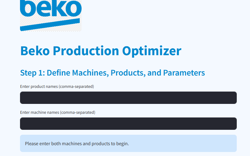
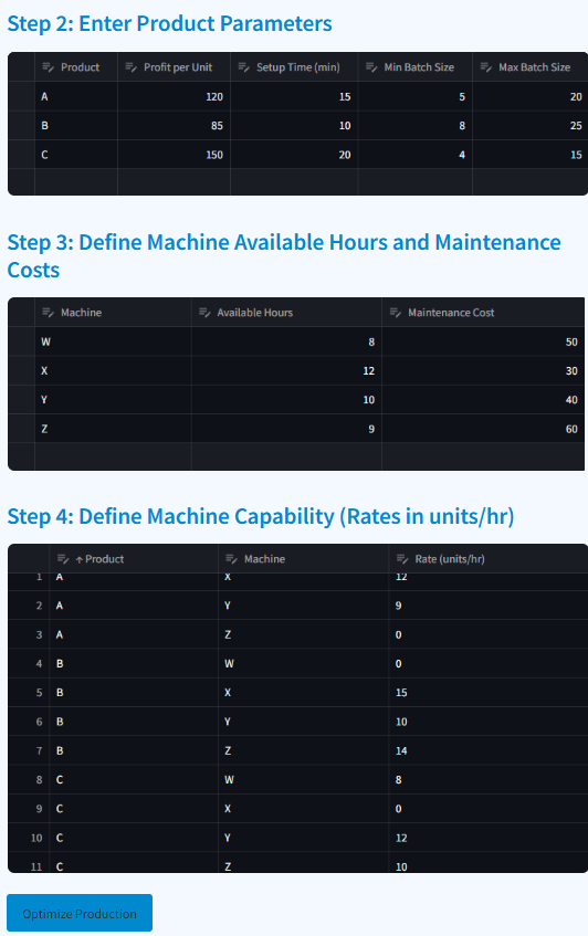
Once the core logic was validated, the focus shifted toward User Experience (UX). By integrating a Streamlit-based frontend, the tool was transformed from a “black box” script into an interactive dashboard. This allows production engineers to input data via structured tables and immediately visualize the impact of changing variables—such as tripling demand for a specific SKU or simulating a machine failure—without modifying the underlying codebase.

❮

🔍 Click to expand

🔍 Click to expand

❯

✕

Technical Details

The system utilizes a decoupled architecture where the Backend executes the heavy lifting of optimization logic via the PuLP library, while the Frontend manages data ingestion and visualization.

The Mathematical Model

The core of the system is an ILP model designed to maximize total profit ($Z$).

Decision Variables:

• $x_{i,j,b}$: Number of batches of Product $i$ on Machine $j$ with batch type $b$ (Integer).
• $y_{i,j,b}$: Binary indicator if Product $i$ is assigned to Machine $j$ with batch type $b$.
• $u_i$: Integer variable representing unmet demand for Product $i$.

Objective Function: The model maximizes profit while subtracting maintenance costs and penalties for unfulfilled orders: $\max Z = \sum_{i} (Profit_i \cdot \sum_{j,b} x_{i,j,b} \cdot BatchSize_{i,b}) - \sum_{i} (Penalty_i \cdot u_i) - \sum_{j,i,b} (Maintenance_j \cdot y_{i,j,b})$

Key Constraints:

1. Machine Time: Ensures production plus setup time does not exceed available hours: $\sum_{i,b} \left( \frac{x_{i,j,b} \cdot BatchSize_{i,b}}{Rate_{i,j}} + SetupTime_i \cdot y_{i,j,b} \right) \leq AvailableHours_j$
2. Batch Exclusivity: Ensures only one batch type (min or max) is selected per product-machine pair.
3. Demand Satisfaction: Ensures the sum of produced units and unmet demand exactly equals the total demand.

Results & Key Metrics

The Production Optimizer successfully handles complex “what-if” scenarios that are computationally difficult to calculate manually:

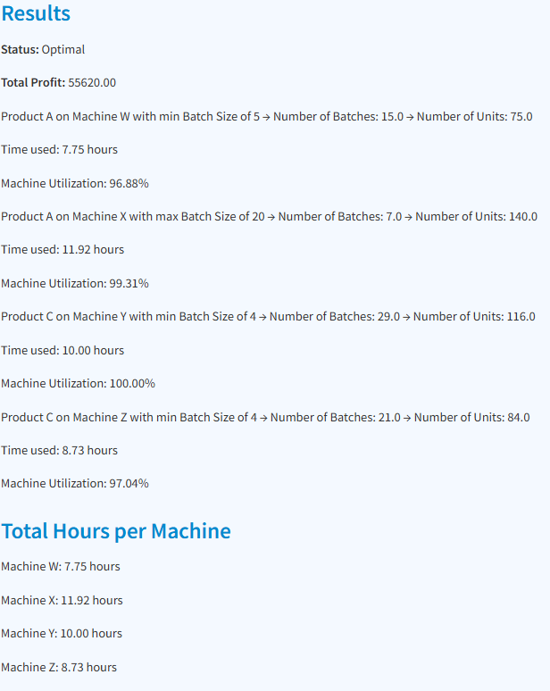
• Scenario A (Standard Operations): The system identifies the optimal distribution of products across machines to maximize profit while remaining within strict machine time limits.

• Scenario B (Machine Failure): By setting a machine’s available hours to zero, the model automatically redistributes the workload across the remaining functional units.

• Scenario C (Demand Surge): When demand for a specific product triples, the system calculates the optimal trade-off between fulfilling high-demand orders and maintaining production of other high-margin items.

Frameworks & Tooling

Python Language

Streamlit Data Visualization

NumPy Computation

Pandas Data Analysis

PuLP Optimization